目录

• 前言
• 一.整体代码结构
• 二.write_txt.py
• 三.yoloData.py
• 四.网络结构
• 五.yoloLoss.py
• 六.train.py
• 七.predict.py
• 八.预测结果

前言

  前面我们介绍了yolov1-v5系列的目标检测理论部分，以及R-CNN，Fast R-CNN，Faster R-CNN，SSD目标检测算法的理论部分，有不懂的小伙伴可以回到前面看看，下面附上链接：

• 目标检测实战篇1——数据集介绍(PASCAL VOC，MS COCO)
  
• YOLOv1目标检测算法——通俗易懂的解析
• YOLOv2目标检测算法——通俗易懂的解析
• YOLOv3目标检测算法——通俗易懂的解析
• YOLOv4目标检测算法——通俗易懂的解析
• YOLOv5目标检测算法——通俗易懂的解析
• R-CNN、Fast RCNN和Faster RCNN网络介绍
• SSD目标检测算法——通俗易懂解析

 这篇博文，我们来详细的剖析下yolov1的代码部分，内容很长，看的过程可能会很艰苦，详细你看完一定会有意想不到的收获。完整的代码放在我的github上了：https://github.com/chasecjg/yolov1

一.整体代码结构

先来看下代码的整体结构，代码没有运行之前主要分为六个文件：

write_txt.py
yoloData.py
new_resnet.py
yoloLoss.py
train.py
predict.py

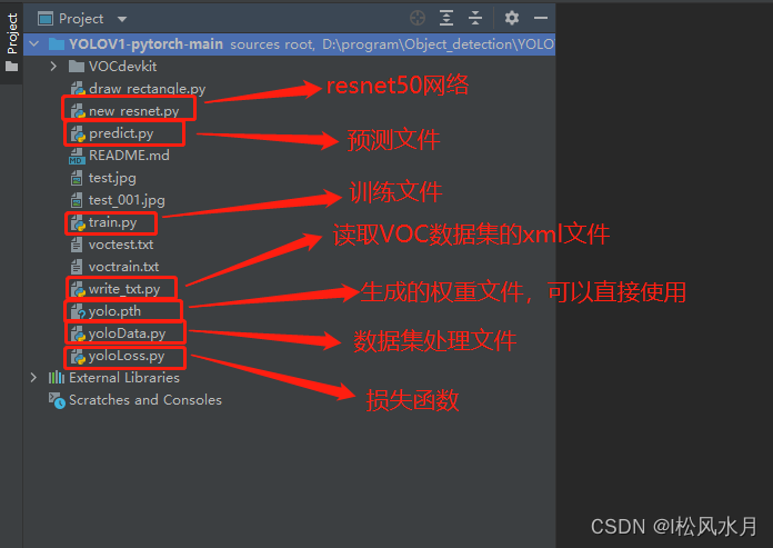
下面我们来逐一解读这六个文件的功能。

二.write_txt.py

  这个代码的作用是用来解析voc数据集的xml文件，在前面介绍数据集的时候我们介绍过voc数据集的标注文件信息内容长什么样。这个脚本的作用就是用来解析这些标注文件，把标注信息中的标注框和类别都给提取出来。我们再来看下这个xml文件里面都是什么信息：

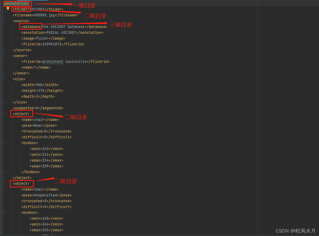
  从上面得xml信息可以看出我们的目标是放在二级目录中的，也就是我们要提取的信息，object下面包含物体的类别，识别难易程度，坐标信息。那我们应该怎么提取这些信息呢？看着很复杂，不要慌，在python中提供了现成的库来解析这些xml信息，就是ElementTree这个库，我们先来简答看下这个库怎么使用的：

class ElementTree:"""ElementTree类是专门解析xml的一个类，在xml.etree.ElementTree包中"""def __init__(self, element=None, file=None):"""element:指的是xml文件的根节点file:指的是已经使用open打开的一个文件对象"""def getroot(self):"""返回树的根节点"""def _setroot(self, element):"""替换根节点"""def parse(self, source, parser=None):"""加载xml文件，解析文件source:是open打开的xml文件的对象parser:是是用什么方式解析xml文件return:返回值是xml文件的根节点"""def iter(self, tag=None):"""创建并返回根标签下所有的元素的迭代器tag:字符串，指的是根标签下的元素的子标签名称，如果不指定，就返回所有的子标签，如果指定只返回该名称的子节点"""# compatibilitydef getiterator(self, tag=None):"""这个方法已经弃用了，使用上面的iter替代"""warnings.warn("This method will be removed in future versions.  ""Use 'tree.iter()' or 'list(tree.iter())' instead.",PendingDeprecationWarning, stacklevel=2)return list(self.iter(tag))def find(self, path, namespaces=None):"""查找名为path标签的内容path:要查找的标签名字"""def findtext(self, path, default=None, namespaces=None):"""根据标记名称或路径找到第一个匹配的元素path:查找的子标签的名称namespace:命名空间返回值是要查找的标签的内容，不存在时返回None"""def findall(self, path, namespaces=None):"""查找所有名为path的子标签的内容path:标签的名称namespace:命名空间返回值是一个list，包含所有的名称为path的子标签的内容"""def iterfind(self, path, namespaces=None):"""根据标记名称找到所有的名为path的子标签的内容，返回值是一个迭代器path:namespace:返回值是一个迭代器"""       def write(self, file_or_filename,encoding=None,xml_declaration=None,default_namespace=None,method=None, *,short_empty_elements=True):

  上面是ElementTree这个类，里面有很多的函数，那么我们怎么利用里面的提供的函数来解析voc数据集的xml文件呢？其实主要用到的就那么几个函数：

 # 加载xml文件，解析文件
parse(self, source, parser=None)
# 查找名为path标签的内容
find(self, path, namespaces=None)
# 查找所有名为path的子标签的内容
findall(self, path, namespaces=None)

  知道了怎么利用ElementTree解析xml文件，下面我们正式进入write_txt.py文件，看看里面是怎么解析的，我们逐个分析，下面再附上这个文件的完整代码，先来看下第一个函数parse，前面用到的参数也放在这了

# 定义一些参数
train_set = open('voctrain.txt', 'w')
test_set = open('voctest.txt', 'w')
Annotations = 'VOCdevkit//VOC2007//Annotations//'
xml_files = os.listdir(Annotations)
random.shuffle(xml_files)  # 打乱数据集
train_num = int(len(xml_files) * 0.7)  # 训练集数量
train_lists = xml_files[:train_num]   # 训练列表
test_lists = xml_files[train_num:]    # 测测试列表def parse_rec(filename):  # 输入xml文件名tree = ET.parse(filename)objects = []# 查找xml文件中所有object元素for obj in tree.findall('object'):# 定义一个字典，存储对象名称和边界信息obj_struct = {}# .text意思是获取文本内容difficult = int(obj.find('difficult').text)if difficult == 1:  # 若为1则跳过本次循环continueobj_struct['name'] = obj.find('name').textbbox = obj.find('bndbox')obj_struct['bbox'] = [int(float(bbox.find('xmin').text)),int(float(bbox.find('ymin').text)),int(float(bbox.find('xmax').text)),int(float(bbox.find('ymax').text))]objects.append(obj_struct)return objects

  上面的代码的功能是，传入要解析的xml文件名，使用ET.parse()方法去解析。查找xml文件中所有的object元素，并将物体类别和位置信息存储在一个字典中。对于每个对象，我们忽略比较难检测的对象。最后，将所有的对象字典存储在一个列表中，并将该列表作为函数的输出返回。接下来，我们再来看下write_txt()函数。
write_txt函数:

def write_txt():count = 0# 生成训练集txtfor train_list in train_lists: count += 1image_name = train_list.split('.')[0] + '.jpg'  # 图片文件名results = parse_rec(Annotations + train_list)# 检查训练集文件是否包含对象if len(results) == 0:print(train_list)continue# 将当前图片文件名写入训练集文本文件train_set.write(image_name)for result in results:class_name = result['name']bbox = result['bbox']# 将当前对象的名称转为其在voc列表中的索引class_name = VOC_CLASSES.index(class_name)train_set.write(' ' + str(bbox[0]) +' ' + str(bbox[1]) +' ' + str(bbox[2]) +' ' + str(bbox[3]) +' ' + str(class_name))train_set.write('\n')train_set.close()# 生成测试集txtfor test_list in test_lists:   count += 1image_name = test_list.split('.')[0] + '.jpg'  # 图片文件名results = parse_rec(Annotations + test_list)if len(results) == 0:print(test_list)continuetest_set.write(image_name)for result in results:class_name = result['name']bbox = result['bbox']class_name = VOC_CLASSES.index(class_name)test_set.write(' ' + str(bbox[0]) +' ' + str(bbox[1]) +' ' + str(bbox[2]) +' ' + str(bbox[3]) +' ' + str(class_name))test_set.write('\n')test_set.close()

  上面这段代码的主要作用是生成训练集和测试集的txt文件，里买保存的都是按照每张图像保存的类别信息和位置信息，一行表示一张图像。把上面两个函数合并，看下完整的代码是什么：

import xml.etree.ElementTree as ET
import os
import randomVOC_CLASSES = (  # 定义所有的类名'aeroplane', 'bicycle', 'bird', 'boat','bottle', 'bus', 'car', 'cat', 'chair','cow', 'diningtable', 'dog', 'horse','motorbike', 'person', 'pottedplant','sheep', 'sofa', 'train', 'tvmonitor')  # 使用其他训练集需要更改# 定义一些参数
train_set = open('voctrain.txt', 'w')
test_set = open('voctest.txt', 'w')
Annotations = 'VOCdevkit//VOC2007//Annotations//'
xml_files = os.listdir(Annotations)
random.shuffle(xml_files)  # 打乱数据集
train_num = int(len(xml_files) * 0.7)  # 训练集数量
train_lists = xml_files[:train_num]  # 训练列表
test_lists = xml_files[train_num:]  # 测测试列表def parse_rec(filename):  # 输入xml文件名tree = ET.parse(filename)objects = []# 查找xml文件中所有object元素for obj in tree.findall('object'):# 定义一个字典，存储对象名称和边界信息obj_struct = {}difficult = int(obj.find('difficult').text)if difficult == 1:  # 若为1则跳过本次循环continueobj_struct['name'] = obj.find('name').textbbox = obj.find('bndbox')obj_struct['bbox'] = [int(float(bbox.find('xmin').text)),int(float(bbox.find('ymin').text)),int(float(bbox.find('xmax').text)),int(float(bbox.find('ymax').text))]objects.append(obj_struct)return objectsdef write_txt():count = 0for train_list in train_lists:  # 生成训练集txtcount += 1image_name = train_list.split('.')[0] + '.jpg'  # 图片文件名results = parse_rec(Annotations + train_list)# 检查训练集文件是否包含对象if len(results) == 0:print(train_list)continue# 将当前图片文件名写入训练集文本文件train_set.write(image_name)for result in results:class_name = result['name']bbox = result['bbox']# 将当前对象的名称转为其在voc列表中的索引class_name = VOC_CLASSES.index(class_name)train_set.write(' ' + str(bbox[0]) +' ' + str(bbox[1]) +' ' + str(bbox[2]) +' ' + str(bbox[3]) +' ' + str(class_name))train_set.write('\n')train_set.close()for test_list in test_lists:  # 生成测试集txtcount += 1image_name = test_list.split('.')[0] + '.jpg'  # 图片文件名results = parse_rec(Annotations + test_list)if len(results) == 0:print(test_list)continuetest_set.write(image_name)for result in results:class_name = result['name']bbox = result['bbox']class_name = VOC_CLASSES.index(class_name)test_set.write(' ' + str(bbox[0]) +' ' + str(bbox[1]) +' ' + str(bbox[2]) +' ' + str(bbox[3]) +' ' + str(class_name))test_set.write('\n')test_set.close()if __name__ == '__main__':write_txt()

  运行上面的代码会生成两个文件，即voctest.txt和voctrain.txt，我们打开voctrain.txt这文件看下这个脚本最后的生成文件长什么样：

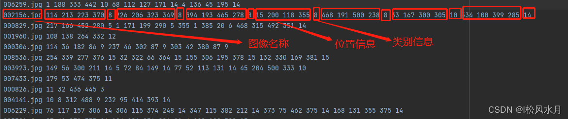
  第二行我们框出来总共7个目标，类别分别为8和14即人和椅子(代码开头有些)，我们来看下对应的原图是不是7个目标：

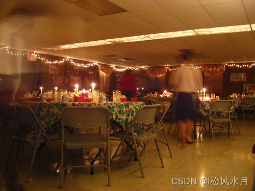
从上面的图中可以看到图中确实是椅子和人，证明我们的标注信息解析是没问题的。

三.yoloData.py

  在write_txt.py文件中，我们已经把每张图的标注信息都已经解析好按行保存在了voctest.txt和voctrain.txt文件中了，接下来就是根据保存的信息来制作标注框了，也就是自定义数据集__init__，__getitem__，__len__这三块内容。下面我们来逐一分析这部分的代码。每行代码都添加了注释。

import pandas as pd
import torch
import cv2
import os
import os.path
import random
import numpy as np
from torch.utils.data import DataLoader, Dataset
from torchvision.transforms import ToTensor
from PIL import Imagepd.set_option('display.max_rows', None)  # ÏÔʾȫ²¿ÐÐ
pd.set_option('display.max_columns', None)  # ÏÔʾȫ²¿ÁÐ# 根据txt文件制作ground truth
CLASS_NUM = 20  # 使用其他训练集需要更改class yoloDataset(Dataset):image_size = 448  # 输入图片大小# list_file为txt文件  img_root为图片路径def __init__(self, img_root, list_file, train, transform):# 初始化参数self.root = img_rootself.train = trainself.transform = transform# 后续要提取txt文件的信息，分类后装入以下三个列表# 文件名self.fnames = []# 位置信息self.boxes = []# 类别信息self.labels = []# 网格大小self.S = 7# 候选框个数self.B = 2# 类别数目self.C = CLASS_NUM# 求均值用的self.mean = (123, 117, 104)# 打开文件，就是voctrain.txt或者voctest.txt文件file_txt = open(list_file)# 读取txt文件每一行lines = file_txt.readlines()# 逐行开始操作for line in lines:# 去除字符串开头和结尾的空白字符，然后按照空白字符（包括空格、制表符、换行符等）分割字符串并返回一个列表splited = line.strip().split()# 存储图片的名字self.fnames.append(splited[0])# 计算一幅图片里面有多少个bbox，注意voctrain.txt或者voctest.txt一行数据只有一张图的信息num_boxes = (len(splited) - 1) // 5# 保存位置信息box = []# 保存标签信息label = []# 提取坐标信息和类别信息for i in range(num_boxes):x = float(splited[1 + 5 * i])y = float(splited[2 + 5 * i])x2 = float(splited[3 + 5 * i])y2 = float(splited[4 + 5 * i])# 提取类别信息，即是20种物体里面的哪一种  值域 0-19c = splited[5 + 5 * i]# 存储位置信息box.append([x, y, x2, y2])# 存储标签信息label.append(int(c))# 解析完所有行的信息后把所有的位置信息放到boxes列表中，boxes里面的是每一张图的坐标信息，也是一个个列表，即形式是[[[x1,y1,x2,y2],[x3,y3,x4,y4]],[[x5,y5,x5,y6]]...]这样的self.boxes.append(torch.Tensor(box))# 形式是[[1,2],[3,4]...]，注意这里是标签，对应位整型数据self.labels.append(torch.LongTensor(label))# 统计图片数量self.num_samples = len(self.boxes)def __getitem__(self, idx):# 获取一张图像fname = self.fnames[idx]# 读取这张图像img = cv2.imread(os.path.join(self.root + fname))# 拷贝一份，避免在对数据进行处理时对原始数据进行修改boxes = self.boxes[idx].clone()labels = self.labels[idx].clone()"""数据增强里面的各种变换用pytorch自带的transform是做不到的，因为对图片进行旋转、随即裁剪等会造成bbox的坐标也会发生变化，所以需要自己来定义数据增强,这里推荐使用功albumentations更简单便捷"""if self.train:img, boxes = self.random_flip(img, boxes)img, boxes = self.randomScale(img, boxes)img = self.randomBlur(img)img = self.RandomBrightness(img)# img = self.RandomHue(img)# img = self.RandomSaturation(img)img, boxes, labels = self.randomShift(img, boxes, labels)# img, boxes, labels = self.randomCrop(img, boxes, labels)#     获取图像高宽信息h, w, _ = img.shape# 归一化位置信息，.expand_as(boxes)的作用是将torch.Tensor([w, h, w, h])扩展成和boxes一样的维度，这样才能进行后面的归一化操作boxes /= torch.Tensor([w, h, w, h]).expand_as(boxes)  # 坐标归一化处理[0,1]，为了方便训练# cv2读取的图像是BGR，转成RGBimg = self.BGR2RGB(img)# 减去均值，帮助网络更快地收敛并提高其性能img = self.subMean(img, self.mean)# 调整图像到统一大小img = cv2.resize(img, (self.image_size, self.image_size))# 将图片标签编码到7x7*30的向量，也就是我们yolov1的最终的输出形式，这个地方不了解的可以去看看yolov1原理target = self.encoder(boxes, labels)# 进行数据增强操作for t in self.transform:img = t(img)# 返回一张图像和所有标注信息return img, targetdef __len__(self):return self.num_samples# 编码图像标签为7x7*30的向量，输入的boxes为一张图的归一化形式位置坐标(X1,Y1,X2,Y2)def encoder(self, boxes, labels):# 网格大小grid_num = 7# 定义一个空的7*7*30的张量target = torch.zeros((grid_num, grid_num, int(CLASS_NUM + 10)))# 对网格进行归一化操作cell_size = 1. / grid_num  # 1/7# 计算每个边框的宽高，wh是一个列表，里面存放的是每一张图的标注框的高宽，形式为[[h1,w1,[h2,w2]...]wh = boxes[:, 2:] - boxes[:, :2]# 每一张图的标注框的中心点坐标，cxcy也是一个列表，形式为[[cx1,cy1],[cx2,cy2]...]cxcy = (boxes[:, 2:] + boxes[:, :2]) / 2# 遍历每个每张图上的标注框信息，cxcy.size()[0]为标注框个数，即计算一张图上几个标注框for i in range(cxcy.size()[0]):# 取中心点坐标cxcy_sample = cxcy[i]# 中心点坐标获取后，计算这个标注框属于哪个grid cell，因为上面归一化了，这里要反归一化，还原回去，坐标从0开始，所以减1，注意坐标从左上角开始ij = (cxcy_sample / cell_size).ceil() - 1# 把标注框框所在的gird cell的的两个bounding box置信度全部置为1，多少行多少列，多少通道的值置为1target[int(ij[1]), int(ij[0]), 4] = 1target[int(ij[1]), int(ij[0]), 9] = 1# 把标注框框所在的gird cell的的两个bounding box类别置为1，这样就完成了该标注框的label信息制作了target[int(ij[1]), int(ij[0]), int(labels[i]) + 10] = 1# 预测框的中心点在图像中的绝对坐标（xy），归一化的xy = ij * cell_size# 标注框的中心点坐标与grid cell左上角坐标的差值，这里又变为了相对于（7*7）的坐标了，目的应该是防止梯度消失，因为这两个值减完后太小了delta_xy = (cxcy_sample - xy) / cell_size# 坐标w,h代表了预测的bounding box的width、height相对于整幅图像width,height的比例# 将目标框的宽高信息存储到target张量中对应的位置上target[int(ij[1]), int(ij[0]), 2:4] = wh[i]  # w1,h1# 目标框的中心坐标相对于所在的grid cell左上角的偏移量保存在target张量中对应的位置上，注意这里保存的是偏移量，并且是相对于（7*7）的坐标，而不是归一的1*1target[int(ij[1]), int(ij[0]), :2] = delta_xy  # x1,y1# 两个bounding box，这里同上target[int(ij[1]), int(ij[0]), 7:9] = wh[i]  # w2,h2target[int(ij[1]), int(ij[0]), 5:7] = delta_xy  # [5,7) 表示x2,y2# 返回制作的标签，可以看到，除了有标注框所在得到位置，其他地方全为0return target  # (xc,yc) = 7*7   (w,h) = 1*1# 以下方法都是数据增强操作，不介绍了，需要注意的是有些增强操作会让图片变形，如仿射变换，这个时候对应的标签也要跟着变化def BGR2RGB(self, img):return cv2.cvtColor(img, cv2.COLOR_BGR2RGB)def BGR2HSV(self, img):return cv2.cvtColor(img, cv2.COLOR_BGR2HSV)def HSV2BGR(self, img):return cv2.cvtColor(img, cv2.COLOR_HSV2BGR)def RandomBrightness(self, bgr):if random.random() < 0.5:hsv = self.BGR2HSV(bgr)h, s, v = cv2.split(hsv)adjust = random.choice([0.5, 1.5])v = v * adjustv = np.clip(v, 0, 255).astype(hsv.dtype)hsv = cv2.merge((h, s, v))bgr = self.HSV2BGR(hsv)return bgrdef RandomSaturation(self, bgr):if random.random() < 0.5:hsv = self.BGR2HSV(bgr)h, s, v = cv2.split(hsv)adjust = random.choice([0.5, 1.5])s = s * adjusts = np.clip(s, 0, 255).astype(hsv.dtype)hsv = cv2.merge((h, s, v))bgr = self.HSV2BGR(hsv)return bgrdef RandomHue(self, bgr):if random.random() < 0.5:hsv = self.BGR2HSV(bgr)h, s, v = cv2.split(hsv)adjust = random.choice([0.5, 1.5])h = h * adjusth = np.clip(h, 0, 255).astype(hsv.dtype)hsv = cv2.merge((h, s, v))bgr = self.HSV2BGR(hsv)return bgrdef randomBlur(self, bgr):if random.random() < 0.5:bgr = cv2.blur(bgr, (5, 5))return bgrdef randomShift(self, bgr, boxes, labels):# 平移变换center = (boxes[:, 2:] + boxes[:, :2]) / 2if random.random() < 0.5:height, width, c = bgr.shapeafter_shfit_image = np.zeros((height, width, c), dtype=bgr.dtype)after_shfit_image[:, :, :] = (104, 117, 123)  # bgrshift_x = random.uniform(-width * 0.2, width * 0.2)shift_y = random.uniform(-height * 0.2, height * 0.2)# print(bgr.shape,shift_x,shift_y)# 原图像的平移if shift_x >= 0 and shift_y >= 0:after_shfit_image[int(shift_y):,int(shift_x):,:] = bgr[:height - int(shift_y),:width - int(shift_x),:]elif shift_x >= 0 and shift_y < 0:after_shfit_image[:height + int(shift_y),int(shift_x):,:] = bgr[-int(shift_y):,:width - int(shift_x),:]elif shift_x < 0 and shift_y >= 0:after_shfit_image[int(shift_y):, :width +int(shift_x), :] = bgr[:height -int(shift_y), -int(shift_x):, :]elif shift_x < 0 and shift_y < 0:after_shfit_image[:height + int(shift_y), :width + int(shift_x), :] = bgr[-int(shift_y):, -int(shift_x):, :]shift_xy = torch.FloatTensor([[int(shift_x), int(shift_y)]]).expand_as(center)center = center + shift_xymask1 = (center[:, 0] > 0) & (center[:, 0] < width)mask2 = (center[:, 1] > 0) & (center[:, 1] < height)mask = (mask1 & mask2).view(-1, 1)boxes_in = boxes[mask.expand_as(boxes)].view(-1, 4)if len(boxes_in) == 0:return bgr, boxes, labelsbox_shift = torch.FloatTensor([[int(shift_x), int(shift_y), int(shift_x), int(shift_y)]]).expand_as(boxes_in)boxes_in = boxes_in + box_shiftlabels_in = labels[mask.view(-1)]return after_shfit_image, boxes_in, labels_inreturn bgr, boxes, labelsdef randomScale(self, bgr, boxes):# 固定住高度，以0.8-1.2伸缩宽度，做图像形变if random.random() < 0.5:scale = random.uniform(0.8, 1.2)height, width, c = bgr.shapebgr = cv2.resize(bgr, (int(width * scale), height))scale_tensor = torch.FloatTensor([[scale, 1, scale, 1]]).expand_as(boxes)boxes = boxes * scale_tensorreturn bgr, boxesreturn bgr, boxesdef randomCrop(self, bgr, boxes, labels):if random.random() < 0.5:center = (boxes[:, 2:] + boxes[:, :2]) / 2height, width, c = bgr.shapeh = random.uniform(0.6 * height, height)w = random.uniform(0.6 * width, width)x = random.uniform(0, width - w)y = random.uniform(0, height - h)x, y, h, w = int(x), int(y), int(h), int(w)center = center - torch.FloatTensor([[x, y]]).expand_as(center)mask1 = (center[:, 0] > 0) & (center[:, 0] < w)mask2 = (center[:, 1] > 0) & (center[:, 1] < h)mask = (mask1 & mask2).view(-1, 1)boxes_in = boxes[mask.expand_as(boxes)].view(-1, 4)if (len(boxes_in) == 0):return bgr, boxes, labelsbox_shift = torch.FloatTensor([[x, y, x, y]]).expand_as(boxes_in)boxes_in = boxes_in - box_shiftboxes_in[:, 0] = boxes_in[:, 0].clamp_(min=0, max=w)boxes_in[:, 2] = boxes_in[:, 2].clamp_(min=0, max=w)boxes_in[:, 1] = boxes_in[:, 1].clamp_(min=0, max=h)boxes_in[:, 3] = boxes_in[:, 3].clamp_(min=0, max=h)labels_in = labels[mask.view(-1)]img_croped = bgr[y:y + h, x:x + w, :]return img_croped, boxes_in, labels_inreturn bgr, boxes, labelsdef subMean(self, bgr, mean):mean = np.array(mean, dtype=np.float32)bgr = bgr - meanreturn bgrdef random_flip(self, im, boxes):if random.random() < 0.5:im_lr = np.fliplr(im).copy()h, w, _ = im.shapexmin = w - boxes[:, 2]xmax = w - boxes[:, 0]boxes[:, 0] = xminboxes[:, 2] = xmaxreturn im_lr, boxesreturn im, boxesdef random_bright(self, im, delta=16):alpha = random.random()if alpha > 0.3:im = im * alpha + random.randrange(-delta, delta)im = im.clip(min=0, max=255).astype(np.uint8)return im

  上面我们分析了yolov1的数据处理部门的代码，其中要注意的一点就是我们在进行数据增强的时候不要忘了对标签也要做处理，不然会导致错误标签。还一个要注意的地方是我们的label中存放的是高宽信息和中心点偏移量信息，其中高宽信息是归一化到[0,1]，中心点相对于grid cell的偏移量是归一化到[0,7]，这里归一化到[0,7]可能是因为这个偏移量太小了，防止在训练的时候出现梯度消失。

四.网络结构

  yolov1的网络结构比较简单，原作者使用的是GoogleNet，我们今天分析的代码使用的是ResNet50，我们知道如果使用448×448×3448\times448\times3448×448×3的图像进行输入的话，那么最终经过ResNet50的输出张量应该是是14×14×204814 \times14 \times204814×14×2048，这显然跟我们需要的输出7×7×307\times7\times307×7×30是不一样的，因此我们需要对网络进行改进，下面我们直接看下改进的代码，然后再放上全部代码：
ResNet50部分代码，在网络的最后输出层增加了基层网络，调整成yolov1的网络输出格式。

class ResNet50(nn.Module):def __init__(self, block):super(ResNet50, self).__init__()self.block = blockself.layer0 = Sequential(Conv2d(3, 64, kernel_size=7, stride=2, padding=3, bias=False),BatchNorm2d(64),ReLU(inplace=True),MaxPool2d(kernel_size=3, stride=2, padding=1))self.layer1 = self.make_layer(self.block, channel=[64, 64], stride1=[1, 1, 1], stride2=[1, 1, 1], n_re=3)self.layer2 = self.make_layer(self.block, channel=[256, 128], stride1=[2, 1, 1], stride2=[1, 1, 1], n_re=4)self.layer3 = self.make_layer(self.block, channel=[512, 256], stride1=[2, 1, 1], stride2=[1, 1, 1], n_re=6)self.layer4 = self.make_layer(self.block, channel=[1024, 512], stride1=[2, 1, 1], stride2=[1, 1, 1], n_re=3)# 调整输出通道self.layer5 = self._make_output_layer(in_channels=2048)# 调整尺寸self.avgpool = nn.AvgPool2d(2)  # kernel_size = 2  , stride = 2# 得到最后输出张量self.conv_end = nn.Conv2d(256, int(CLASS_NUM + 10), kernel_size=3, stride=1, padding=1, bias=False)self.bn_end = nn.BatchNorm2d(int(CLASS_NUM + 10))def make_layer(self, block, channel, stride1, stride2, n_re):layers = []for num_layer in range(0, n_re):if num_layer == 0:layers.append(block(channel[0], channel[1], stride1, downsample=True))else:layers.append(block(channel[1]*4, channel[1], stride2, downsample=False))return Sequential(*layers)def _make_output_layer(self, in_channels):layers = []layers.append(output_net(in_planes=in_channels,planes=256,block_type='B'))layers.append(output_net(in_planes=256,planes=256,block_type='A'))layers.append(output_net(in_planes=256,planes=256,block_type='A'))return nn.Sequential(*layers)def forward(self, x):# print(x.shape) # 3*448*448out = self.layer0(x)# print(out.shape) # 64*112*112out = self.layer1(out)# print(out.shape)  # 256*112*112out = self.layer2(out)# print(out.shape) # 512*56*56out = self.layer3(out)# print(out.shape) # 1024*28*28out = self.layer4(out)  # 2048*14*14out = self.layer5(out)  # batch_size*256*14*14out = self.avgpool(out)  # batch_size*256*7*7out = self.conv_end(out)  # batch_size*30*7*7out = self.bn_end(out)out = torch.sigmoid(out)out = out.permute(0, 2, 3, 1)  # bitch_size*7*7*30return out

output_net部分代码：

class output_net(nn.Module):# no expansion# dilation = 2# type B use 1x1 convexpansion = 1def __init__(self, in_planes, planes, stride=1, block_type='A'):super(output_net, self).__init__()self.conv1 = nn.Conv2d(in_planes, planes, kernel_size=1, bias=False)self.bn1 = nn.BatchNorm2d(planes)self.conv2 = nn.Conv2d(planes, planes, kernel_size=3, stride=stride, padding=2, bias=False, dilation=2)self.bn2 = nn.BatchNorm2d(planes)self.conv3 = nn.Conv2d(planes, self.expansion * planes, kernel_size=1, bias=False)self.bn3 = nn.BatchNorm2d(self.expansion * planes)self.downsample = nn.Sequential()self.relu = nn.ReLU(inplace=True)if stride != 1 or in_planes != self.expansion * planes or block_type == 'B':self.downsample = nn.Sequential(nn.Conv2d(in_planes,self.expansion * planes,kernel_size=1,stride=stride,bias=False),nn.BatchNorm2d(self.expansion * planes))def forward(self, x):out = self.relu(self.bn1(self.conv1(x)))out = self.relu(self.bn2(self.conv2(out)))out = self.bn3(self.conv3(out))out += self.downsample(x)out = self.relu(out)return out

  代码部分没什么好分析的，比较简单，就是在ResNet50的最后输出层接几层网络让其变成yolov1的输出格式7×7×307\times7\times307×7×30。实在看不懂的可以评论区留言解答。

五.yoloLoss.py

  下面我们来详细解释下损失函数部分，代码里面每句话都做了非常详细的注释。

import torch
import torch.nn as nn
import torch.nn.functional as F
from torch.autograd import Variable
import warningswarnings.filterwarnings('ignore')  # 忽略警告消息
CLASS_NUM = 20    # （使用自己的数据集时需要更改）class yoloLoss(nn.Module):def __init__(self, S, B, l_coord, l_noobj):# 一般而言 l_coord = 5 ， l_noobj = 0.5super(yoloLoss, self).__init__()# 网格数self.S = S  # S = 7# bounding box数量self.B = B  # B = 2# 权重系数self.l_coord = l_coord# 权重系数self.l_noobj = l_noobjdef compute_iou(self, box1, box2):  # box1(2,4)  box2(1,4)N = box1.size(0)  # 2M = box2.size(0)  # 1lt = torch.max(  # 返回张量所有元素的最大值# [N,2] -> [N,1,2] -> [N,M,2]box1[:, :2].unsqueeze(1).expand(N, M, 2),# [M,2] -> [1,M,2] -> [N,M,2]box2[:, :2].unsqueeze(0).expand(N, M, 2),)rb = torch.min(# [N,2] -> [N,1,2] -> [N,M,2]box1[:, 2:].unsqueeze(1).expand(N, M, 2),# [M,2] -> [1,M,2] -> [N,M,2]box2[:, 2:].unsqueeze(0).expand(N, M, 2),)wh = rb - lt  # [N,M,2]wh[wh < 0] = 0  # clip at 0inter = wh[:, :, 0] * wh[:, :, 1]  # [N,M]  重复面积area1 = (box1[:, 2] - box1[:, 0]) * (box1[:, 3] - box1[:, 1])  # [N,]area2 = (box2[:, 2] - box2[:, 0]) * (box2[:, 3] - box2[:, 1])  # [M,]area1 = area1.unsqueeze(1).expand_as(inter)  # [N,] -> [N,1] -> [N,M]area2 = area2.unsqueeze(0).expand_as(inter)  # [M,] -> [1,M] -> [N,M]iou = inter / (area1 + area2 - inter)# iou的形状是(2,1)，里面存放的是两个框的iou的值return iou  # [2,1]def forward(self, pred_tensor, target_tensor):'''pred_tensor: (tensor) size(batchsize,7,7,30)target_tensor: (tensor) size(batchsize,7,7,30)，就是在yoloData中制作的标签'''# batchsize大小N = pred_tensor.size()[0]# 判断目标在哪个网格，输出B*7*7的矩阵，有目标的地方为True，其他地方为false,这里就用了第4位，第9位和第4位一样就没判断coo_mask = target_tensor[:, :, :, 4] > 0# 判断目标不在那个网格，输出B*7*7的矩阵，没有目标的地方为True，其他地方为falsenoo_mask = target_tensor[:, :, :, 4] == 0# 将 coo_mask tensor 在最后一个维度上增加一维，并将其扩展为与 target_tensor tensor 相同的形状，得到含物体的坐标等信息，大小为batchsize*7*7*30coo_mask = coo_mask.unsqueeze(-1).expand_as(target_tensor)# 将 noo_mask 在最后一个维度上增加一维，并将其扩展为与 target_tensor tensor 相同的形状，得到不含物体的坐标等信息，大小为batchsize*7*7*30noo_mask = noo_mask.unsqueeze(-1).expand_as(target_tensor)# 根据label的信息从预测的张量取出对应位置的网格的30个信息按照出现序号拼接成以一维张量，这里只取包含目标的coo_pred = pred_tensor[coo_mask].view(-1, int(CLASS_NUM + 10))# 所有的box的位置坐标和置信度放到box_pred中，塑造成X行5列（-1表示自动计算），一个box包含5个值box_pred = coo_pred[:, :10].contiguous().view(-1, 5)# 类别信息class_pred = coo_pred[:, 10:]  # [n_coord, 20]# pred_tensor[coo_mask]把pred_tensor中有物体的那个网格对应的30个向量拿出来，这里对应的是label向量，只计算有目标的coo_target = target_tensor[coo_mask].view(-1, int(CLASS_NUM + 10))box_target = coo_target[:, :10].contiguous().view(-1, 5)class_target = coo_target[:, 10:]# 不包含物体grid ceil的置信度损失,这里是label的输出的向量。noo_pred = pred_tensor[noo_mask].view(-1, int(CLASS_NUM + 10))noo_target = target_tensor[noo_mask].view(-1, int(CLASS_NUM + 10))# 创建一个跟noo_pred相同形状的张量，形状为（x,30），里面都是全0或全1，再使用bool将里面的0或1转为true和falsenoo_pred_mask = torch.cuda.ByteTensor(noo_pred.size()).bool()# 把创建的noo_pred_mask全部改成false，因为这里对应的是没有目标的张量noo_pred_mask.zero_()# 把不包含目标的张量的置信度位置置为1noo_pred_mask[:, 4] = 1noo_pred_mask[:, 9] = 1# 跟上面的pred_tensor[coo_mask]一个意思，把不包含目标的置信度提取出来拼接成一维张量noo_pred_c = noo_pred[noo_pred_mask]# 同noo_pred_cnoo_target_c = noo_target[noo_pred_mask]# 计算loss，让预测的值越小越好，因为不包含目标，置信度越为0越好nooobj_loss = F.mse_loss(noo_pred_c, noo_target_c, size_average=False)  # 均方误差# 注意：上面计算的不包含目标的损失只计算了置信度，其他的都没管"""计算包含目标的损失：位置损失+类别损失"""# 先创建两个张量用于后面匹配预测的两个编辑框：一个负责预测，一个不负责预测# 创建一跟box_target相同的张量,这里用来匹配后面负责预测的框coo_response_mask = torch.cuda.ByteTensor(box_target.size()).bool()# 全部置为Falsecoo_response_mask.zero_()  # 全部元素置False# 创建一跟box_target相同的张量，这里用来匹配不负责预测的框no_coo_response_mask = torch.cuda.ByteTensor(box_target.size()).bool()# 全部置为Falseno_coo_response_mask.zero_()# 创建一个全0张量，匹配后面的预测框的ioubox_target_iou = torch.zeros(box_target.size()).cuda()# 遍历每一个标注框，每次遍历两个是因为一个标注框对应有两个预测框要跟他匹配，box1 = 预测框  box2 = ground truth# box_target.size()[0]：有多少bbox，并且一次取两个bbox，因为两个bbox才是一个完整的预测框for i in range(0, box_target.size()[0], 2):  ##  第i个grid ceil对应的两个bboxbox1 = box_pred[i:i + 2]# 创建一个和box1大小(2,5)相同的浮点型张量用来存储坐标，这里代码使用的torch版本可能比较老，其实Variable可以省略的box1_xyxy = Variable(torch.FloatTensor(box1.size()))# box1_xyxy[:, :2]为预测框中心点坐标相对于所在grid cell左上角的偏移，前面在数据处理的时候讲过label里面的值是归一化为(0-7)的，# 因此这里得反归一化成跟宽高一样比例，归一化到(0-1),减去宽高的一半得到预测框的左上角的坐标相对于他所在的grid cell的左上角的偏移量box1_xyxy[:, :2] = box1[:, :2] / float(self.S) - 0.5 * box1[:, 2:4]# 计算右下角坐标相对于预测框所在的grid cell的左上角的偏移量box1_xyxy[:, 2:4] = box1[:, :2] / float(self.S) + 0.5 * box1[:, 2:4]# target中的两个框的目标信息是一模一样的，这里取其中一个就行了box2 = box_target[i].view(-1, 5)box2_xyxy = Variable(torch.FloatTensor(box2.size()))box2_xyxy[:, :2] = box2[:, :2] / float(self.S) - 0.5 * box2[:, 2:4]box2_xyxy[:, 2:4] = box2[:, :2] / float(self.S) + 0.5 * box2[:, 2:4]# 计算两个预测框与标注框的IoU值，返回计算结果，是个列表iou = self.compute_iou(box1_xyxy[:, :4], box2_xyxy[:, :4])# 通过max()函数获取与gt最大的框的iou和索引号(第几个框)max_iou, max_index = iou.max(0)# 将max_index放到GPU上max_index = max_index.data.cuda()# 保留IoU比较大的那个框coo_response_mask[i + max_index] = 1  # IOU最大的bbox# 舍去的bbox,两个框单独标记为1，分开存放，方便下面计算no_coo_response_mask[i + 1 - max_index] = 1# 将预测框比较大的IoU的那个框保存在box_target_iou中，# 其中i + max_index表示当前预测框对应的位置，torch.LongTensor([4]).cuda()表示在box_target_iou中存储最大IoU的值的位置。box_target_iou[i + max_index, torch.LongTensor([4]).cuda()] = max_iou.data.cuda()# 放到GPU上box_target_iou = Variable(box_target_iou).cuda()# 负责预测物体的预测框的位置信息（含物体的grid ceil的两个bbox与ground truth的IOU较大的一方）box_pred_response = box_pred[coo_response_mask].view(-1, 5)# 标注信息，拿出来一个计算就行了，因为两个信息一模一样box_target_response_iou = box_target_iou[coo_response_mask].view(-1, 5)# IOU较小的一方no_box_pred_response = box_pred[no_coo_response_mask].view(-1, 5)no_box_target_response_iou = box_target_iou[no_coo_response_mask].view(-1, 5)# 不负责预测物体的置信度置为0，本来就是0，这里有点多此一举no_box_target_response_iou[:, 4] = 0# 负责预测物体的标注框对应的label的信息box_target_response = box_target[coo_response_mask].view(-1, 5)# 包含物的体grid ceil中IOU较大的bbox置信度损失contain_loss = F.mse_loss(box_pred_response[:, 4], box_target_response_iou[:, 4], size_average=False)# 不包含物体的grid ceil中舍去的bbox的置信度损失no_contain_loss = F.mse_loss(no_box_pred_response[:, 4], no_box_target_response_iou[:, 4], size_average=False)# 负责预测物体的预测框的位置损失loc_loss = F.mse_loss(box_pred_response[:, :2], box_target_response[:, :2], size_average=False) + F.mse_loss(torch.sqrt(box_pred_response[:, 2:4]), torch.sqrt(box_target_response[:, 2:4]), size_average=False)# 负责预测物体的所在grid cell的类别损失class_loss = F.mse_loss(class_pred, class_target, size_average=False)# 计算总损失，这里有个权重return (self.l_coord * loc_loss + contain_loss + self.l_noobj * (nooobj_loss + no_contain_loss) + class_loss) / N

其中有几个点需要注意一下，当时也是卡了很久才看明白，我们先来看下这个函数：

coo_pred = pred_tensor[coo_mask].view(-1, int(CLASS_NUM + 10))

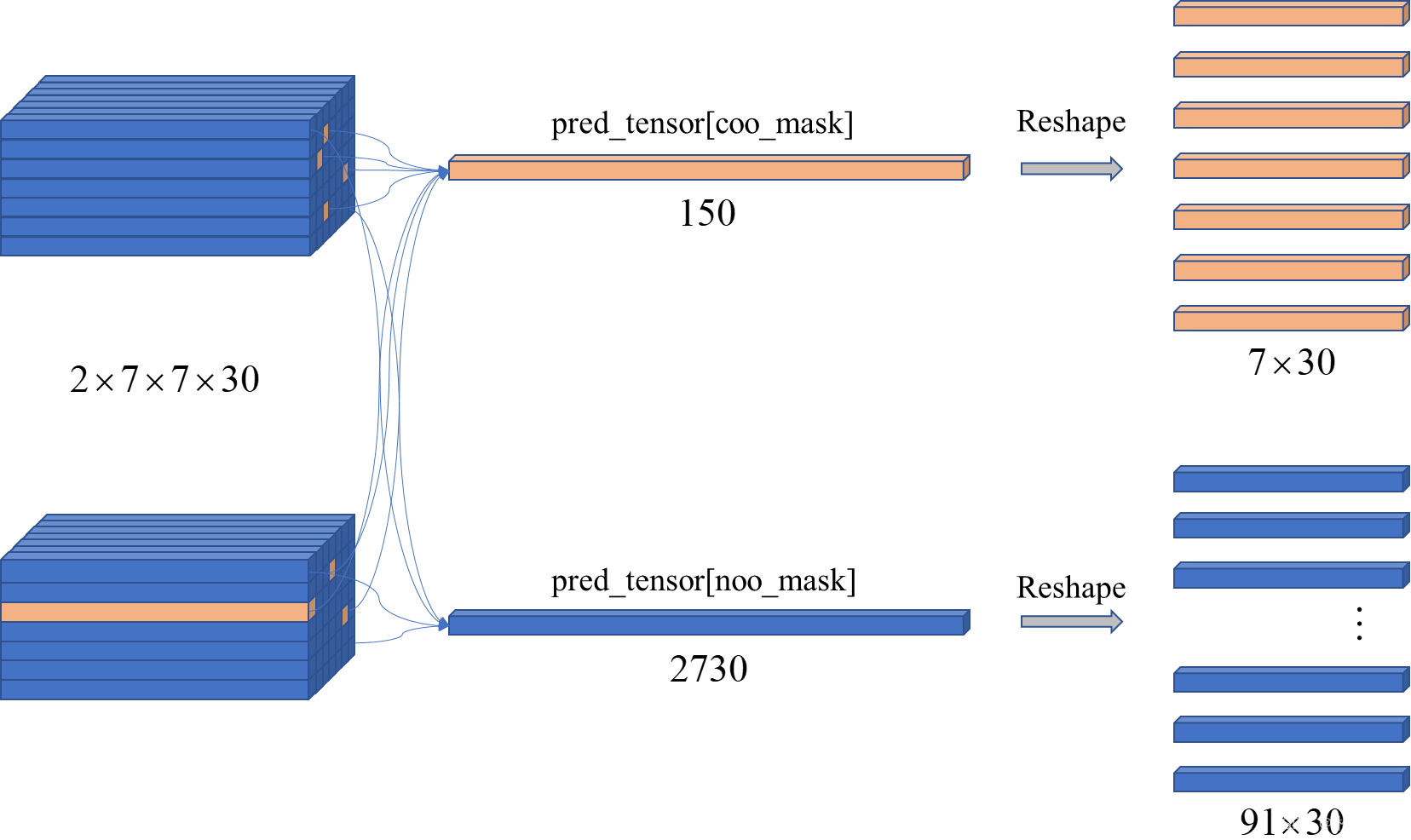
  我来根据上面的图解释下这句话，其中coo_mask是一个跟pred_tensor一样大小的张量，里面存放的是True和False，执行完pred_tensor[coo_mask]这个函数之后就会把coo_mask里面为True的位置的元素在pred_tensor提取出来，按照先后顺序拼接成一个一维张量，最后再reshape，提取出包含目标的向量和不包含目标的向量。
还一个地方是计算偏移量的时候：

# box1_xyxy[:, :2]为预测框中心点坐标相对于所在grid cell左上角的偏移，前面在数据处理的时候讲过label里面的值是归一化为(0-7)的，
# 因此这里得反归一化成跟宽高一样比例，归一化到(0-1),减去宽高的一半得到预测框的左上角的坐标相对于他所在的grid cell的左上角的偏移量
box1_xyxy[:, :2] = box1[:, :2] / float(self.S) - 0.5 * box1[:, 2:4]
# 计算右下角坐标相对于预测框所在的grid cell的左上角的偏移量
box1_xyxy[:, 2:4] = box1[:, :2] / float(self.S) + 0.5 * box1[:, 2:4]
# target中的两个框的目标信息是一模一样的，这里取其中一个就行了
box2 = box_target[i].view(-1, 5)
box2_xyxy = Variable(torch.FloatTensor(box2.size()))
box2_xyxy[:, :2] = box2[:, :2] / float(self.S) - 0.5 * box2[:, 2:4]
box2_xyxy[:, 2:4] = box2[:, :2] / float(self.S) + 0.5 * box2[:, 2:4]

  上面计算偏移量的时候一定是针对预测框所在的grid cell的左上角的偏移，以及预测框的中心点坐标是相对于grid cell的左上角的偏移并且按照(0-7)的归一化，因为label是归一化到(0-7)，所以在计算的时候要反归一化跟宽高一样都是(0-1)。

六.train.py

  上面介绍了损失函数部分的代码，下面开始进入训练阶段了，已经在代码中做了逐行注释。

from yoloData import yoloDataset
from yoloLoss import yoloLoss
from new_resnet import resnet50
from torchvision import models
import torchvision.transforms as transforms
from torch.utils.data import DataLoader
import torchdevice = 'cuda'
file_root = 'VOCdevkit/VOC2007/JPEGImages/'
batch_size = 4
learning_rate = 0.001
num_epochs = 100# 自定义训练数据集
train_dataset = yoloDataset(img_root=file_root, list_file='voctrain.txt', train=True, transform=[transforms.ToTensor()])
# 加载自定义的训练数据集
train_loader = DataLoader(train_dataset, batch_size=batch_size, shuffle=True, num_workers=0)
# 自定义测试数据集
test_dataset = yoloDataset(img_root=file_root, list_file='voctest.txt', train=False, transform=[transforms.ToTensor()])
# 加载自定义的测试数据集
test_loader = DataLoader(test_dataset, batch_size=batch_size, shuffle=True, num_workers=0)
print('the dataset has %d images' % (len(train_dataset)))"""
下面这段代码主要适用于迁移学习训练，可以将预训练的ResNet-50模型的参数赋值给新的网络，以加快训练速度和提高准确性。
"""
# 创建改编的ResNet50
net = resnet50()
# 放到GPU上
net = net.cuda()
# 直接使用pytorch加载resnet50,带预训练权重
resnet = models.resnet50(pretrained=True)  # torchvison库中的网络
# 获取resnet的训练参数
new_state_dict = resnet.state_dict()
# 获取刚创建的改编的resnet50()的参数
op = net.state_dict()# 无论名称是否相同都可以使用
for new_state_dict_num, new_state_dict_value in enumerate(new_state_dict.values()):# op.keys()表示获取模型参数字典中的所有键值for op_num, op_key in enumerate(op.keys()):# 320个key中不需要最后的全连接层的两个参数if op_num == new_state_dict_num and op_num <= 317:op[op_key] = new_state_dict_value
# 将预训练好的参数放入改编的ResNet的网络中，加快训练速度
net.load_state_dict(op)print('cuda', torch.cuda.current_device(), torch.cuda.device_count())   # 确认一下cuda的设备# 创建损失函数
criterion = yoloLoss(7, 2, 5, 0.5)
# 放到GPU上
criterion = criterion.to(device)
# 训练前需要加入的语句，一般有Dropout()的时候要加
net.train()# 里面存字典
params = []
# net.named_parameters()是一个PyTorch函数，它返回一个包含模型中所有需要学习的参数（即权重和偏置项）及其名称的迭代器。
params_dict = dict(net.named_parameters())
for key, value in params_dict.items():# 把字典放到列表中，这个“+”可以理解为appendparams += [{'params': [value], 'lr':learning_rate}]# 定义优化器  “随机梯度下降”
optimizer = torch.optim.SGD(# 上面已经将模型参数打包成字典了，这里不需要用net.parameters()了params,# 学习率lr=learning_rate,# 动量momentum=0.9,# 正则化weight_decay=5e-4)# Windows环境下使用多进程时需要调用的函数，我训练的时候没用。在Windows下使用多进程需要先将Python脚本打包成exe文件，而freeze_support()的作用就是冻结可执行文件的代码，确保在Windows下正常运行多进程。
# torch.multiprocessing.freeze_support()  # 多进程相关 猜测是使用多显卡训练需要
"""这里解释下自己定义参数列表和直接使用net.parameter()的区别：在大多数情况下，直接使用net.parameters()和将模型参数放到字典中是没有区别的，因为net.parameters()本身就是一个包含模型所有参数的列表。但是，如果我们想要对不同的参数设置不同的超参数，那么将模型参数放到字典中会更加方便。使用net.parameters()的话，我们需要手动区分不同的参数，再分别进行超参数的设置。而将模型参数放到字典中后，我们可以直接对每个参数设置对应的超参数，更加简洁和灵活。举个例子，如果我们想要对卷积层和全连接层设置不同的学习率，使用net.parameters()的话，我们需要手动区分哪些参数属于卷积层，哪些参数属于全连接层，然后分别对这两部分参数设置不同的学习率。而将模型参数放到字典中后，我们可以直接对卷积层和全连接层的参数分别设置不同的学习率，更加方便和清晰。
"""
# 开始训练
for epoch in range(num_epochs):# 这个地方形成习惯，因为网络可能会用到Dropout和batchnormnet.train()# 调整学习率if epoch == 60:learning_rate = 0.0001if epoch == 80:learning_rate = 0.00001# optimizer.param_groups 返回一个包含优化器参数分组信息的列表，每个分组是一个字典，主要包含以下键值：# params：当前参数分组中需要更新的参数列表，如网络的权重，偏置等。# lr：当前参数分组的学习率。就是我们要提取更新的# momentum：当前参数分组的动量参数。# weight_decay：当前参数分组的权重衰减参数。for param_group in optimizer.param_groups:param_group['lr'] = learning_rate      # 更改全部的学习率print('\n\nStarting epoch %d / %d' % (epoch + 1, num_epochs))print('Learning Rate for this epoch: {}'.format(learning_rate))# 计算损失total_loss = 0.# 开始迭代训练for i, (images, target) in enumerate(train_loader):images, target = images.cuda(), target.cuda()pred = net(images)# 创建损失函数loss = criterion(pred, target)total_loss += loss.item()# 梯度清零optimizer.zero_grad()# 反向传播loss.backward()# 参数优化optimizer.step()if (i + 1) % 5 == 0:print('Epoch [%d/%d], Iter [%d/%d] Loss: %.4f, average_loss: %.4f' % (epoch +1, num_epochs, i + 1, len(train_loader), loss.item(), total_loss / (i + 1)))# 开始测试validation_loss = 0.0net.eval()for i, (images, target) in enumerate(test_loader):images, target = images.cuda(), target.cuda()# 输入图像pred = net(images)# 计算损失loss = criterion(pred, target)# 累加损失validation_loss += loss.item()# 计算平均lossvalidation_loss /= len(test_loader)best_test_loss = validation_lossprint('get best test loss %.5f' % best_test_loss)# 保存模型参数torch.save(net.state_dict(), 'yolo.pth')

七.predict.py

  模型训练完之后就到了我们的测试阶段，同上面一样，每行代码都做了详细的解释，下面附上代码：

import numpy as np
import torch
from PIL import ImageFont, ImageDraw
from cv2 import cv2
from matplotlib import pyplot as plt
# import cv2
from torchvision.transforms import ToTensorfrom draw_rectangle import draw
from new_resnet import resnet50# voc数据集的类别信息，这里转换成字典形式
classes = {"aeroplane": 0, "bicycle": 1, "bird": 2, "boat": 3, "bottle": 4, "bus": 5, "car": 6, "cat": 7, "chair": 8, "cow": 9, "diningtable": 10, "dog": 11, "horse": 12, "motorbike": 13, "person": 14, "pottedplant": 15, "sheep": 16, "sofa": 17, "train": 18, "tvmonitor": 19}# 测试图片的路径
img_root = "D:\\program\\Object_detection\\YOLOV1-pytorch-main\\test.jpg"
# 网络模型
model = resnet50()
# 加载权重，就是在train.py中训练生成的权重文件yolo.pth
model.load_state_dict(torch.load("D:\\program\\Object_detection\\YOLOV1-pytorch-main\\yolo.pth"))
# 测试模式
model.eval()
# 设置置信度
confident = 0.2
# 设置iou阈值
iou_con = 0.4# 类别信息，这里写的都是voc数据集的，如果是自己的数据集需要更改
VOC_CLASSES = ('aeroplane', 'bicycle', 'bird', 'boat','bottle', 'bus', 'car', 'cat', 'chair','cow', 'diningtable', 'dog', 'horse','motorbike', 'person', 'pottedplant','sheep', 'sofa', 'train', 'tvmonitor')
# 类别总数：20
CLASS_NUM = len(VOC_CLASSES)"""
注意：预测和训练的时候是不同的，训练的时候是有标签参考的，在测试的时候会直接输出两个预测框，
保留置信度比较大的，再通过NMS处理得到最终的预测结果，不要跟训练阶段搞混了
"""# target 7*7*30  值域为0-1
class Pred():# 参数初始化def __init__(self, model, img_root):self.model = modelself.img_root = img_rootdef result(self):# 读取测试的图像img = cv2.imread(self.img_root)# 获取高宽信息h, w, _ = img.shape# 调整图像大小image = cv2.resize(img, (448, 448))# CV2读取的图像是BGR，这里转回RGB模式img = cv2.cvtColor(image, cv2.COLOR_BGR2RGB)# 图像均值mean = (123, 117, 104)  # RGB# 减去均值进行标准化操作img = img - np.array(mean, dtype=np.float32)# 创建数据增强函数transform = ToTensor()# 图像转为tensor，因为cv2读取的图像是numpy格式img = transform(img)# 输入要求是BCHW，加一个batch维度img = img.unsqueeze(0)# 图像输入模型，返回值为1*7*7*30的张量Result = self.model(img)# 获取目标的边框信息bbox = self.Decode(Result)# 非极大值抑制处理bboxes = self.NMS(bbox)    # n*6   bbox坐标是基于7*7网格需要将其转换成448# draw(image, bboxes, classes)if len(bboxes) == 0:print("未识别到任何物体")print("尝试减小 confident 以及 iou_con")print("也可能是由于训练不充分，可在训练时将epoch增大")        for i in range(0, len(bboxes)):    # bbox坐标将其转换为原图像的分辨率bboxes[i][0] = bboxes[i][0] * 64bboxes[i][1] = bboxes[i][1] * 64bboxes[i][2] = bboxes[i][2] * 64bboxes[i][3] = bboxes[i][3] * 64x1 = bboxes[i][0].item()    # 后面加item()是因为画框时输入的数据不可一味tensor类型x2 = bboxes[i][1].item()y1 = bboxes[i][2].item()y2 = bboxes[i][3].item()class_name = bboxes[i][5].item()print(x1, x2, y1, y2, VOC_CLASSES[int(class_name)])cv2.rectangle(image, (int(x1), int(y1)), (int(x2), int(y2)), (144, 144, 255))   # 画框plt.imsave('test_001.jpg', image)# cv2.imwrite("img", image)# cv2.imshow('img', image)# cv2.waitKey(0)# 接受的result的形状为1*7*7*30def Decode(self, result):# 去掉batch维度result = result.squeeze()# 提取置信度信息，并在最后一个维度增加一维，跟后面匹配result[:, :, 4]的形状为7*7,最后变为7*7*1grid_ceil1 = result[:, :, 4].unsqueeze(2)# 同上grid_ceil2 = result[:, :, 9].unsqueeze(2)# 两个置信度信息按照维度2拼接grid_ceil_con = torch.cat((grid_ceil1, grid_ceil2), 2)# 按照第二个维度进行最大值求取，一个grid ceil两个bbox，两个confidence，也就是找置信度比较大的那个，形状都是7*7grid_ceil_con, grid_ceil_index = grid_ceil_con.max(2)# 找出一个gird cell中预测类别最大的物体的索引和预测条件类别概率class_p, class_index = result[:, :, 10:].max(2)# 计算出物体的真实概率，类别最大的物体乘上置信度比较大的那个框得到最终的真实物体类别概率class_confidence = class_p * grid_ceil_con# 定义一个张量，记录位置信息bbox_info = torch.zeros(7, 7, 6)for i in range(0, 7):for j in range(0, 7):# 获取置信度比较大的索引位置bbox_index = grid_ceil_index[i, j]# 把置信度比较大的那个框的位置信息保存到bbox_info中，另一个直接抛弃bbox_info[i, j, :5] = result[i, j, (bbox_index * 5):(bbox_index+1) * 5]# 真实目标概率bbox_info[:, :, 4] = class_confidence# 类别信息bbox_info[:, :, 5] = class_index# 返回预测的结果,7*7*6    6 = bbox4个信息+类别概率+类别代号return bbox_info# 非极大值抑制处理，按照类别处理，bbox为Decode获取的预测框的位置信息和类别概率和类别信息def NMS(self, bbox, iou_con=iou_con):for i in range(0, 7):for j in range(0, 7):# xc = bbox[i, j, 0]# yc = bbox[i, j, 1]# w = bbox[i, j, 2] * 7# h = bbox[i, j, 3] * 7# Xc = i + xc# Yc = j + yc# xmin = Xc - w/2# xmax = Xc + w/2# ymin = Yc - h/2# ymax = Yc + h/2# 注意，目前bbox的四个坐标是以grid ceil的左上角为坐标原点，而且单位不一致中心点偏移的坐标是归一化为(0-7),宽高是(0-7),，单位不一致，全部归一化为(0-7)# 计算预测框的左上角右下角相对于7*7网格的位置xmin = j + bbox[i, j, 0] - bbox[i, j, 2] * 7 / 2     # xminxmax = j + bbox[i, j, 0] + bbox[i, j, 2] * 7 / 2     # xmaxymin = i + bbox[i, j, 1] - bbox[i, j, 3] * 7 / 2     # yminymax = i + bbox[i, j, 1] + bbox[i, j, 3] * 7 / 2     # ymaxbbox[i, j, 0] = xminbbox[i, j, 1] = xmaxbbox[i, j, 2] = yminbbox[i, j, 3] = ymax# 调整形状，bbox本来就是(49*6)，这里感觉没必要bbox = bbox.view(-1, 6)# 存放最终需要保留的预测框bboxes = []# 取出每个gird cell中的类别信息，返回一个列表ori_class_index = bbox[:, 5]# 按照类别进行排序，从高到低，返回的是排序后的类别列表和对应的索引位置,如下："""类别排序tensor([ 1.,  1.,  1.,  1.,  1.,  1.,  1.,  2.,  2.,  2.,  2.,  2.,  2.,  2.,3.,  3.,  3.,  4.,  4.,  4.,  4.,  5.,  5.,  5.,  6.,  6.,  6.,  6.,6.,  6.,  6.,  6.,  7.,  8.,  8.,  8.,  8.,  8., 14., 14., 14., 14.,14., 14., 14., 15., 15., 16., 17.], grad_fn=)位置索引tensor([48, 47, 46, 45, 44, 43, 42,  7,  8, 22, 11, 16, 14, 15, 24, 20,  1,  2,6,  0, 13, 23, 25, 27, 32, 39, 38, 35, 33, 31, 30, 28,  3, 26, 10, 19,9, 12, 29, 41, 40, 21, 37, 36, 34, 18, 17,  5,  4])"""class_index, class_order = ori_class_index.sort(dim=0, descending=False)# class_index是一个tensor，这里把他转为列表形式class_index = class_index.tolist()# 根据排序后的索引更改bbox排列顺序bbox = bbox[class_order, :]a = 0for i in range(0, CLASS_NUM):# 统计目标数量，即某个类别出现在grid cell中的次数num = class_index.count(i)# 预测框中没有这个类别就直接跳过if num == 0:continue# 提取同一类别的所有信息x = bbox[a:a+num, :]# 提取真实类别概率信息score = x[:, 4]# 提取出来的某一类别按照真实类别概率信息高度排序，递减score_index, score_order = score.sort(dim=0, descending=True)# 根据排序后的结果更改真实类别的概率排布y = x[score_order, :]# 先看排在第一位的物体的概率是否大有给定的阈值，不满足就不看这个类别了，丢弃全部的预测框if y[0, 4] >= confident:for k in range(0, num):# 真实类别概率，排序后的y_score = y[:, 4]# 对真实类别概率重新排序，保证排列顺序依照递减，其实跟上面一样的，多此一举_, y_score_order = y_score.sort(dim=0, descending=True)y = y[y_score_order, :]# 判断概率是否大于0if y[k, 4] > 0:# 计算预测框的面积area0 = (y[k, 1] - y[k, 0]) * (y[k, 3] - y[k, 2])for j in range(k+1, num):# 计算剩余的预测框的面积area1 = (y[j, 1] - y[j, 0]) * (y[j, 3] - y[j, 2])x1 = max(y[k, 0], y[j, 0])x2 = min(y[k, 1], y[j, 1])y1 = max(y[k, 2], y[j, 2])y2 = min(y[k, 3], y[j, 3])w = x2 - x1h = y2 - y1if w < 0 or h < 0:w = 0h = 0inter = w * h# 计算与真实目标概率最大的那个框的iouiou = inter / (area0 + area1 - inter)# iou大于一定值则认为两个bbox识别了同一物体删除置信度较小的bbox# 同时物体类别概率小于一定值也认为不包含物体if iou >= iou_con or y[j, 4] < confident:y[j, 4] = 0for mask in range(0, num):if y[mask, 4] > 0:bboxes.append(y[mask])# 进入下个类别a = num + a#     返回最终预测的框return bboxesif __name__ == "__main__":Pred = Pred(model, img_root)Pred.result()

我对上面的NMS部分的几句代码进行解释下：

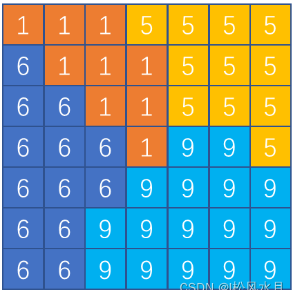
num = class_index.count(i)# 预测框中没有这个类别就直接跳过if num == 0:continue

  要知道一张图里面可能就几个目标，十几个目标，一个目标是要占一片区域的，这个区域的grid cell的类别就是这个物体的类别，上面的代码的目的就是统计某个类别的网格数目，然后再进行非极大值抑制处理。

八.预测结果

下面展示一下预测结果：

至此，关于yolov1的代码解析部分已经全部介绍完了，如有错误，敬请指正。完整的代码在我的github上可以下载到：https://github.com/chasecjg/yolov1